
In this section, we apply our software to the graphical representation of some results from the theory of curves.
Curves in two-dimensional space may be given by an equation
|
f(x1,x2) = 0 |
|
x (t) = (x1(t),x2(t)) (t Î I Ì R). |
Example 4. Some algebraic curves
Figure 10. The geometric definition of a double egg line
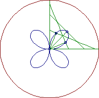
Figure 11. The geometric definition of a rosette
Now we study envelopes of families of curves.
Let I Ì R be an interval and G = {gc:c Î I} be a family of curves in a plane, given by the equations
|
f(x1,x2; c) = 0 for c Î I. |
|
¶F/¶c (x1,x2; c) = 0. |
Example 5. The envelope of a family of ellipses
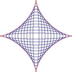
Figure 12. A family of curves (p-norm) and their envelope; a = 2

Figure 13. A family of curves (p-norm) and their envelope; a = 4

Figure 14. A family of curves (p-norm) and their envelope; a = 3/4
Now we consider orthogonal trajectories. Let G = {gc: c Î I} be a family of curves that cover a domain D Ì R2 such that there is one and only one curve through every point of D. The curves g^ that intersect every curve gc Î G at a right angle are called orthogonal trajectories of G. If the curves gc are given by the equation f(x1,x2; c) = 0, then the orthogonal trajectories are given by the solutions of the differential equations
|
dx2/dx1 ¶f /¶x1 (x1,x2; c) = ¶f /¶x2(x1,x2; c). |
Example 6. Orthogonal trajectories of generalized circle lines
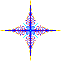
Figure 15. A family of curves (p-norm) and their orthogonal trajectories; a = 1/2
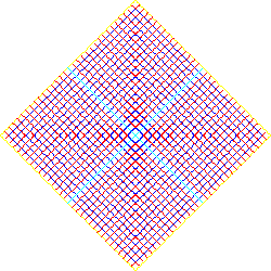
Figure 16. A family of curves (p-norm) and their orthogonal trajectories; a = 1
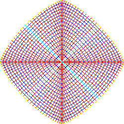
Figure 17. A family of curves (p-norm) and their orthogonal trajectories; a = 4/3
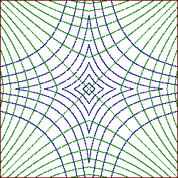
Figure 18. A family of curves (metric) and their orthogonal trajectories
In this part we deal with the graphical representation of some results from the general theory of curves.
Let g be a curve in three-dimensional Euclidean space R3 with a parametric representation
x(s) = (x1(s),x2(x),x3(s)) with s the arc length along g.
Then the vectors
v1(s) = x'(s)
v2(s) = x''(s)
/ || x''(s) || and
v3(s) = v1(s)
× v2(s).
Example 7. The vectors of the trihedra of a helix with a parametric representation
x(s) = (r cos(w s), r sin(w s), h w s) with s Î R where r > 0, h Î R and w = 1 / (r2+h2)1/2 arc constants.
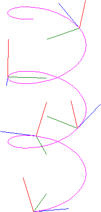
Figure 19. The vectors of trihedra of a helix
The vector x''(s) and its length k(s) = || x''(s) || are called the vector of curvature and the curvature of g at s. The curvature is a measure of the deviation of a curve from a straight line. The uniquely defined circle in the osculating plane of a curve g at s, which is a second order approximation of g at s, is called the osculating circle of g at s.
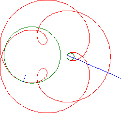
Figure 20. Vectors of curvature and osculating circles
The value t(s) = v'2(s) · v3(s) is called the torsion of g at s. The torsion is a measure of the deviation of a curve from a plane.
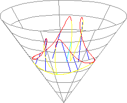
Figure 21. The torsion along a non-planar curve on a cone
Example 8. The curvature and torsion of the helix in Example 7 are given by k(s) = rw2 and t(s) = hw2. The third order approximations of the helix in the osculating, normal and rectifying planes are given by the equations
y=1/2 r w2x2,
z2 = 2/9 h2 / r · w
2y3 and
z = 1/6 r h w4x3,
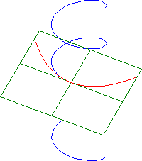
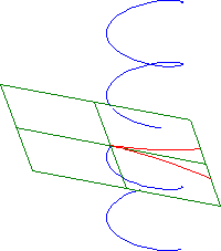
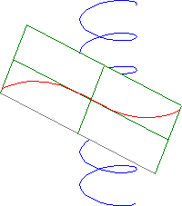
Figure 22. Third order approximations of a helix in the osculation, normal and rectifying planes
Let g be a curve with a parametric representation x(s). Then the osculating sphere of g at s is the sphere that is a third order approximation of g at s. The osculating sphere of a curve g at s is uniquely defined whenever k(s), t(s) ¹ 0; its centre and radius are given by
m(s) = x(s) + v2(s) / k(s) - k'(s)v3(s) / t(s)
and
r(s) = ( 1/k2(s) + (k'(s))2/ (t2(s) k4(s)) )1/2
Example 9. The osculating sphere of the helix in Example 7 is given by
m(s) =
( -h2/r cos(ws),
-h2/r sin(ws),
hws )
and
r(s) = (r2+h2)/r.
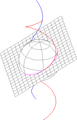
Figure 23. Helix with osculating plane and osculating sphere
The fundamental theorem of curves states that the shape of a curve is uniquely defined by its curvature and torsion.
Example 10. Planar curves with k(s) = c·s where c is a constant are klothoids. Planar curves with k(s) = c/Ös where c is a constant are the lines of intersections of a helix with a plane orthogonal to the axis of the helix.
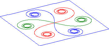
Figure 24. A curve with k(s) = c·s
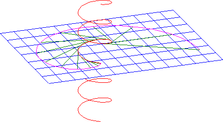
Figure 25. A curve with k(s) = c/Ös
Curves with the property that their curvature and torsion are proportional are called lines of constant slope; they have a constant angle with a given direction in space.
Example 11. Lines of constant slope on surfaces of revolution.

Figure 26. Orthogonal projections of lines of constant slope on a sphere and a paraboloid of rotation on to planes